
Rha Overstreet - PharaohSun
# Importing libraries
import pandas as pd
import numpy as np
import seaborn as sns
import matplotlib.pyplot as plt
from statsmodels.formula.api import ols as sm_ols
from statsmodels.iolib.summary2 import summary_col # nicer tables
# Reading in dataset
df = pd.read_csv('input_data2/housing_train.csv')
Part 1: EDA
Simple EDA
def edaSimple(df):
    numerics = ['int16', 'int32', 'int64', 'float16', 'float32', 'float64']
    numeric_variables = df.select_dtypes(include=numerics).columns
    categorical_variables = df.drop(numeric_variables, axis = 1).columns
    dataShape = df.shape
    num_unique = df[numeric_variables].nunique()
    cat_unique = df[categorical_variables].nunique()
    units_of_observation = ['v_SalePrice', 'v_Year_Built','v_Yr_Sold','v_Mo_Sold', 'v_Lot_Area']

    print("There are", df.shape[0], "observations and", df.shape[1], "variables.", "\n",
         "The build dates range from", df.v_Year_Built.min(), "to", df.v_Year_Built.max(), "\n",
         "The sale dates range from", df.v_Yr_Sold.min(), "to", df.v_Yr_Sold.max(), "\n")

    print("The shape of the data is", "\n", dataShape, "\n",
         "Numeric Variables", "\n", numeric_variables , "\n",
         "Categorical Variables", "\n", categorical_variables , "\n",
         "Number of unique numerical variables", "\n", num_unique , "\n",
         "Number of unique categorical variables", "\n", cat_unique , "\n",
         "Main units of observation", "\n", df[units_of_observation].describe(), "\n",
         "Categorical variable counts", "\n")

    for var in categorical_variables:
            print(var, "| Note: limited to top 5 values.")
            print(df[var].value_counts().head(5), '\n---')
edaSimple(df)
There are 1941 observations and 81 variables.
 The build dates range from 1872 to 2008
 The sale dates range from 2006 to 2008

The shape of the data is
 (1941, 81)
 Numeric Variables
 Index(['v_MS_SubClass', 'v_Lot_Frontage', 'v_Lot_Area', 'v_Overall_Qual',
       'v_Overall_Cond', 'v_Year_Built', 'v_Year_Remod/Add', 'v_Mas_Vnr_Area',
       'v_BsmtFin_SF_1', 'v_BsmtFin_SF_2', 'v_Bsmt_Unf_SF', 'v_Total_Bsmt_SF',
       'v_1st_Flr_SF', 'v_2nd_Flr_SF', 'v_Low_Qual_Fin_SF', 'v_Gr_Liv_Area',
       'v_Bsmt_Full_Bath', 'v_Bsmt_Half_Bath', 'v_Full_Bath', 'v_Half_Bath',
       'v_Bedroom_AbvGr', 'v_Kitchen_AbvGr', 'v_TotRms_AbvGrd', 'v_Fireplaces',
       'v_Garage_Yr_Blt', 'v_Garage_Cars', 'v_Garage_Area', 'v_Wood_Deck_SF',
       'v_Open_Porch_SF', 'v_Enclosed_Porch', 'v_3Ssn_Porch', 'v_Screen_Porch',
       'v_Pool_Area', 'v_Misc_Val', 'v_Mo_Sold', 'v_Yr_Sold', 'v_SalePrice'],
      dtype='object')
 Categorical Variables
 Index(['parcel', 'v_MS_Zoning', 'v_Street', 'v_Alley', 'v_Lot_Shape',
       'v_Land_Contour', 'v_Utilities', 'v_Lot_Config', 'v_Land_Slope',
       'v_Neighborhood', 'v_Condition_1', 'v_Condition_2', 'v_Bldg_Type',
       'v_House_Style', 'v_Roof_Style', 'v_Roof_Matl', 'v_Exterior_1st',
       'v_Exterior_2nd', 'v_Mas_Vnr_Type', 'v_Exter_Qual', 'v_Exter_Cond',
       'v_Foundation', 'v_Bsmt_Qual', 'v_Bsmt_Cond', 'v_Bsmt_Exposure',
       'v_BsmtFin_Type_1', 'v_BsmtFin_Type_2', 'v_Heating', 'v_Heating_QC',
       'v_Central_Air', 'v_Electrical', 'v_Kitchen_Qual', 'v_Functional',
       'v_Fireplace_Qu', 'v_Garage_Type', 'v_Garage_Finish', 'v_Garage_Qual',
       'v_Garage_Cond', 'v_Paved_Drive', 'v_Pool_QC', 'v_Fence',
       'v_Misc_Feature', 'v_Sale_Type', 'v_Sale_Condition'],
      dtype='object')
 Number of unique numerical variables
 v_MS_SubClass          16
v_Lot_Frontage        118
v_Lot_Area           1413
v_Overall_Qual         10
v_Overall_Cond          9
v_Year_Built          110
v_Year_Remod/Add       60
v_Mas_Vnr_Area        368
v_BsmtFin_SF_1        787
v_BsmtFin_SF_2        194
v_Bsmt_Unf_SF         938
v_Total_Bsmt_SF       870
v_1st_Flr_SF          901
v_2nd_Flr_SF          508
v_Low_Qual_Fin_SF      23
v_Gr_Liv_Area        1045
v_Bsmt_Full_Bath        3
v_Bsmt_Half_Bath        3
v_Full_Bath             4
v_Half_Bath             3
v_Bedroom_AbvGr         8
v_Kitchen_AbvGr         3
v_TotRms_AbvGrd        13
v_Fireplaces            5
v_Garage_Yr_Blt        99
v_Garage_Cars           5
v_Garage_Area         520
v_Wood_Deck_SF        306
v_Open_Porch_SF       230
v_Enclosed_Porch      147
v_3Ssn_Porch           20
v_Screen_Porch         96
v_Pool_Area            14
v_Misc_Val             28
v_Mo_Sold              12
v_Yr_Sold               3
v_SalePrice           820
dtype: int64
 Number of unique categorical variables
 parcel              1941
v_MS_Zoning            7
v_Street               2
v_Alley                2
v_Lot_Shape            4
v_Land_Contour         4
v_Utilities            2
v_Lot_Config           5
v_Land_Slope           3
v_Neighborhood        28
v_Condition_1          9
v_Condition_2          8
v_Bldg_Type            5
v_House_Style          8
v_Roof_Style           6
v_Roof_Matl            8
v_Exterior_1st        16
v_Exterior_2nd        17
v_Mas_Vnr_Type         5
v_Exter_Qual           4
v_Exter_Cond           5
v_Foundation           6
v_Bsmt_Qual            5
v_Bsmt_Cond            5
v_Bsmt_Exposure        4
v_BsmtFin_Type_1       6
v_BsmtFin_Type_2       6
v_Heating              6
v_Heating_QC           5
v_Central_Air          2
v_Electrical           5
v_Kitchen_Qual         4
v_Functional           8
v_Fireplace_Qu         5
v_Garage_Type          6
v_Garage_Finish        3
v_Garage_Qual          5
v_Garage_Cond          5
v_Paved_Drive          3
v_Pool_QC              4
v_Fence                4
v_Misc_Feature         5
v_Sale_Type           10
v_Sale_Condition       6
dtype: int64
 Main units of observation
          v_SalePrice  v_Year_Built    v_Yr_Sold    v_Mo_Sold     v_Lot_Area
count    1941.000000   1941.000000  1941.000000  1941.000000    1941.000000
mean   182033.238022   1971.321999  2006.998454     6.431221   10284.770222
std     80407.100395     30.209933     0.801736     2.745199    7832.295527
min     13100.000000   1872.000000  2006.000000     1.000000    1470.000000
25%    130000.000000   1953.000000  2006.000000     5.000000    7420.000000
50%    161900.000000   1973.000000  2007.000000     6.000000    9450.000000
75%    215000.000000   2001.000000  2008.000000     8.000000   11631.000000
max    755000.000000   2008.000000  2008.000000    12.000000  164660.000000
 Categorical variable counts

parcel | Note: limited to top 5 values.
1056_528110080    1
1124_528477040    1
1108_528365080    1
1107_528365060    1
1105_528363020    1
Name: parcel, dtype: int64
---
v_MS_Zoning | Note: limited to top 5 values.
RL         1499
RM          320
FV           87
RH           17
C (all)      15
Name: v_MS_Zoning, dtype: int64
---
v_Street | Note: limited to top 5 values.
Pave    1933
Grvl       8
Name: v_Street, dtype: int64
---
v_Alley | Note: limited to top 5 values.
Grvl    82
Pave    54
Name: v_Alley, dtype: int64
---
v_Lot_Shape | Note: limited to top 5 values.
Reg    1213
IR1     661
IR2      55
IR3      12
Name: v_Lot_Shape, dtype: int64
---
v_Land_Contour | Note: limited to top 5 values.
Lvl    1736
HLS      90
Bnk      77
Low      38
Name: v_Land_Contour, dtype: int64
---
v_Utilities | Note: limited to top 5 values.
AllPub    1940
NoSewr       1
Name: v_Utilities, dtype: int64
---
v_Lot_Config | Note: limited to top 5 values.
Inside     1431
Corner      326
CulDSac     119
FR2          53
FR3          12
Name: v_Lot_Config, dtype: int64
---
v_Land_Slope | Note: limited to top 5 values.
Gtl    1850
Mod      81
Sev      10
Name: v_Land_Slope, dtype: int64
---
v_Neighborhood | Note: limited to top 5 values.
NAmes      290
CollgCr    183
OldTown    155
Edwards    129
Somerst    121
Name: v_Neighborhood, dtype: int64
---
v_Condition_1 | Note: limited to top 5 values.
Norm      1674
Feedr      111
Artery      55
RRAn        39
PosN        21
Name: v_Condition_1, dtype: int64
---
v_Condition_2 | Note: limited to top 5 values.
Norm      1918
Feedr        9
Artery       4
PosN         3
PosA         3
Name: v_Condition_2, dtype: int64
---
v_Bldg_Type | Note: limited to top 5 values.
1Fam      1607
TwnhsE     158
Twnhs       66
Duplex      64
2fmCon      46
Name: v_Bldg_Type, dtype: int64
---
v_House_Style | Note: limited to top 5 values.
1Story    968
2Story    581
1.5Fin    212
SLvl       85
SFoyer     54
Name: v_House_Style, dtype: int64
---
v_Roof_Style | Note: limited to top 5 values.
Gable      1543
Hip         356
Gambrel      16
Flat         15
Mansard       7
Name: v_Roof_Style, dtype: int64
---
v_Roof_Matl | Note: limited to top 5 values.
CompShg    1908
Tar&Grv      16
WdShake       7
WdShngl       6
Membran       1
Name: v_Roof_Matl, dtype: int64
---
v_Exterior_1st | Note: limited to top 5 values.
VinylSd    670
MetalSd    308
HdBoard    293
Wd Sdng    277
Plywood    136
Name: v_Exterior_1st, dtype: int64
---
v_Exterior_2nd | Note: limited to top 5 values.
VinylSd    666
MetalSd    310
HdBoard    266
Wd Sdng    263
Plywood    180
Name: v_Exterior_2nd, dtype: int64
---
v_Mas_Vnr_Type | Note: limited to top 5 values.
None       1154
BrkFace     602
Stone       146
BrkCmn       20
CBlock        1
Name: v_Mas_Vnr_Type, dtype: int64
---
v_Exter_Qual | Note: limited to top 5 values.
TA    1201
Gd     658
Ex      65
Fa      17
Name: v_Exter_Qual, dtype: int64
---
v_Exter_Cond | Note: limited to top 5 values.
TA    1704
Gd     187
Fa      41
Ex       8
Po       1
Name: v_Exter_Cond, dtype: int64
---
v_Foundation | Note: limited to top 5 values.
PConc     882
CBlock    813
BrkTil    210
Slab       28
Stone       6
Name: v_Foundation, dtype: int64
---
v_Bsmt_Qual | Note: limited to top 5 values.
TA    847
Gd    817
Ex    168
Fa     57
Po      2
Name: v_Bsmt_Qual, dtype: int64
---
v_Bsmt_Cond | Note: limited to top 5 values.
TA    1723
Gd      93
Fa      70
Ex       3
Po       2
Name: v_Bsmt_Cond, dtype: int64
---
v_Bsmt_Exposure | Note: limited to top 5 values.
No    1227
Av     292
Gd     203
Mn     167
Name: v_Bsmt_Exposure, dtype: int64
---
v_BsmtFin_Type_1 | Note: limited to top 5 values.
Unf    577
GLQ    549
ALQ    292
Rec    197
BLQ    172
Name: v_BsmtFin_Type_1, dtype: int64
---
v_BsmtFin_Type_2 | Note: limited to top 5 values.
Unf    1666
Rec      68
LwQ      61
BLQ      40
ALQ      33
Name: v_BsmtFin_Type_2, dtype: int64
---
v_Heating | Note: limited to top 5 values.
GasA    1913
GasW      18
Grav       4
Wall       3
OthW       2
Name: v_Heating, dtype: int64
---
v_Heating_QC | Note: limited to top 5 values.
Ex    993
TA    553
Gd    333
Fa     59
Po      3
Name: v_Heating_QC, dtype: int64
---
v_Central_Air | Note: limited to top 5 values.
Y    1812
N     129
Name: v_Central_Air, dtype: int64
---
v_Electrical | Note: limited to top 5 values.
SBrkr    1771
FuseA     127
FuseF      34
FuseP       7
Mix         1
Name: v_Electrical, dtype: int64
---
v_Kitchen_Qual | Note: limited to top 5 values.
TA    994
Gd    771
Ex    132
Fa     44
Name: v_Kitchen_Qual, dtype: int64
---
v_Functional | Note: limited to top 5 values.
Typ     1813
Min1      42
Min2      40
Mod       22
Maj1      15
Name: v_Functional, dtype: int64
---
v_Fireplace_Qu | Note: limited to top 5 values.
Gd    504
TA    388
Fa     50
Po     31
Ex     28
Name: v_Fireplace_Qu, dtype: int64
---
v_Garage_Type | Note: limited to top 5 values.
Attchd     1143
Detchd      520
BuiltIn     122
Basment      21
2Types       20
Name: v_Garage_Type, dtype: int64
---
v_Garage_Finish | Note: limited to top 5 values.
Unf    813
RFn    536
Fin    485
Name: v_Garage_Finish, dtype: int64
---
v_Garage_Qual | Note: limited to top 5 values.
TA    1719
Fa      89
Gd      20
Po       4
Ex       2
Name: v_Garage_Qual, dtype: int64
---
v_Garage_Cond | Note: limited to top 5 values.
TA    1758
Fa      50
Gd      14
Po      10
Ex       2
Name: v_Garage_Cond, dtype: int64
---
v_Paved_Drive | Note: limited to top 5 values.
Y    1751
N     147
P      43
Name: v_Paved_Drive, dtype: int64
---
v_Pool_QC | Note: limited to top 5 values.
Ex    4
Gd    4
TA    3
Fa    2
Name: v_Pool_QC, dtype: int64
---
v_Fence | Note: limited to top 5 values.
MnPrv    210
GdPrv     76
GdWo      69
MnWw      10
Name: v_Fence, dtype: int64
---
v_Misc_Feature | Note: limited to top 5 values.
Shed    55
Gar2     4
Othr     2
Elev     1
TenC     1
Name: v_Misc_Feature, dtype: int64
---
v_Sale_Type | Note: limited to top 5 values.
WD       1647
New       201
COD        51
ConLD      16
CWD        12
Name: v_Sale_Type, dtype: int64
---
v_Sale_Condition | Note: limited to top 5 values.
Normal     1551
Partial     205
Abnorml     127
Family       34
Alloca       12
Name: v_Sale_Condition, dtype: int64
---
Graphs
sns.scatterplot(data = df, x = 'v_Year_Built', y = 'v_SalePrice',
                hue = 'v_Neighborhood', palette = "mako", alpha = 0.7)
plt.legend(bbox_to_anchor=(1.02, 1), loc='upper left', borderaxespad=0, ncol = 2)
<matplotlib.legend.Legend at 0x7f8ca8a6bee0>
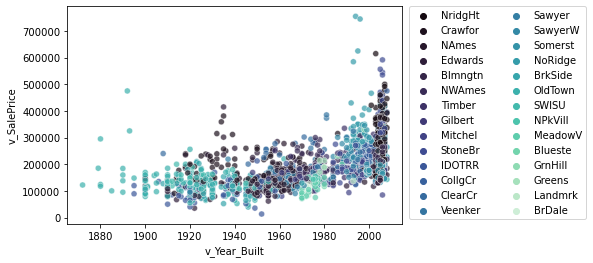
Note - all PairGrid plots have the same hue meanings. Legend will only be displayed for one for brevity.
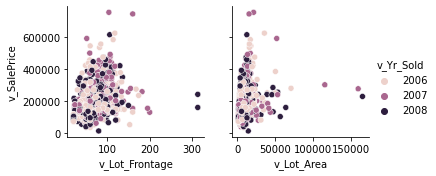
lot_vars = ['v_Lot_Frontage', 'v_Lot_Area']
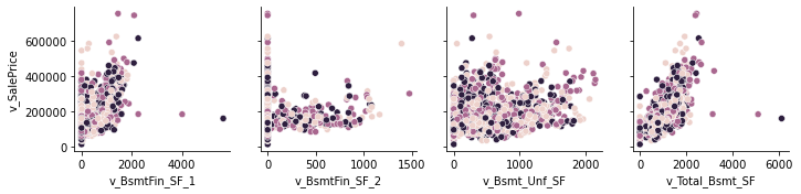
bmnt_vars = ['v_BsmtFin_SF_1', 'v_BsmtFin_SF_2', 'v_Bsmt_Unf_SF', 'v_Total_Bsmt_SF']
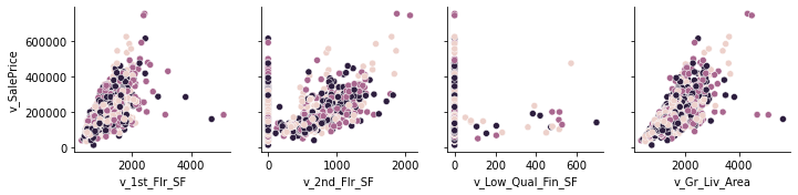
flr_vars = ['v_1st_Flr_SF', 'v_2nd_Flr_SF', 'v_Low_Qual_Fin_SF', 'v_Gr_Liv_Area']
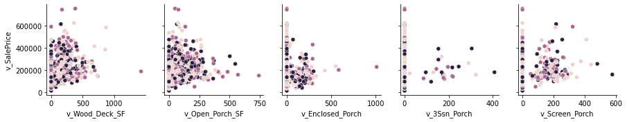
out_vars = ['v_Wood_Deck_SF','v_Open_Porch_SF', 'v_Enclosed_Porch',
'v_3Ssn_Porch', 'v_Screen_Porch']
a = sns.PairGrid(df, x_vars = lot_vars, y_vars = 'v_SalePrice', hue = 'v_Yr_Sold')
a.map(sns.scatterplot)
a.add_legend()
<seaborn.axisgrid.PairGrid at 0x7f8c912ac6a0>
b = sns.PairGrid(df, x_vars = bmnt_vars, y_vars = 'v_SalePrice', hue = 'v_Yr_Sold')
b.map(sns.scatterplot)
<seaborn.axisgrid.PairGrid at 0x7f8c907e9af0>
c = sns.PairGrid(df, x_vars = flr_vars, y_vars = 'v_SalePrice', hue = 'v_Yr_Sold')
c.map(sns.scatterplot)
<seaborn.axisgrid.PairGrid at 0x7f8c916df760>
b = sns.PairGrid(df, x_vars = out_vars, y_vars = 'v_SalePrice', hue = 'v_Yr_Sold')
b.map(sns.scatterplot)
<seaborn.axisgrid.PairGrid at 0x7f8c913f1d90>
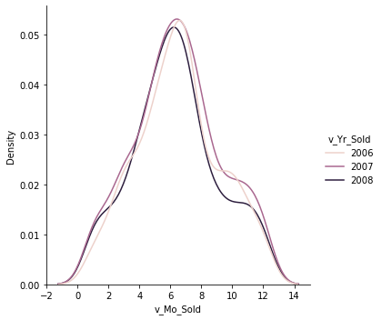
sns.displot(data = df, x = 'v_Mo_Sold', kind = 'kde', hue = 'v_Yr_Sold')
<seaborn.axisgrid.FacetGrid at 0x7f8c916df5e0>
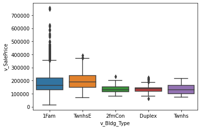
sns.boxplot(data = df, x = 'v_Bldg_Type', y = 'v_SalePrice')
<AxesSubplot:xlabel='v_Bldg_Type', ylabel='v_SalePrice'>
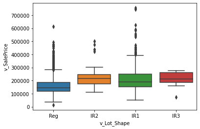
sns.boxplot(data = df, x = 'v_Lot_Shape', y = 'v_SalePrice')
<AxesSubplot:xlabel='v_Lot_Shape', ylabel='v_SalePrice'>
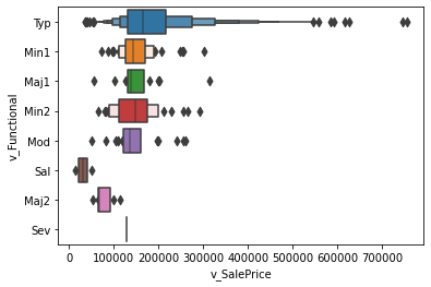
sns.boxenplot(data = df, x = 'v_SalePrice', y = 'v_Functional')
<AxesSubplot:xlabel='v_SalePrice', ylabel='v_Functional'>
Part 2: Running Regressions
Run these regressions on the RAW data, even if you found data issues that you think should be addressed.
Insert cells as needed below to run these regressions. Note that $i$ is indexing a given house, and $t$ indexes the year of sale.
- $\text{Sale Price}_{i,t} = \alpha + \beta_1 * \text{v_Lot_Area}$
- $\text{Sale Price}_{i,t} = \alpha + \beta_1 * log(\text{v_Lot_Area})$
- $log(\text{Sale Price}_{i,t}) = \alpha + \beta_1 * \text{v_Lot_Area}$
- $log(\text{Sale Price}_{i,t}) = \alpha + \beta_1 * log(\text{v_Lot_Area})$
- $log(\text{Sale Price}_{i,t}) = \alpha + \beta_1 * \text{v_Yr_Sold}$
- $log(\text{Sale Price}_{i,t}) = \alpha + \beta_1 * (\text{v_Yr_Sold==2007})+ \beta_2 * (\text{v_Yr_Sold==2008})$
- Choose your own adventure: Pick any five variables from the dataset that you think will generate good R2. Use them in a regression of $log(\text{Sale Price}_{i,t})$
- Tip: You can transform/create these five variables however you want, even if it creates extra variables. For example: I’d count Model 6 above as only using one variable:
v_Yr_Sold. - I got an R2 of 0.877 with just “5” variables. How close can you get? I won’t be shocked if someone beats that!
- Tip: You can transform/create these five variables however you want, even if it creates extra variables. For example: I’d count Model 6 above as only using one variable:
Bonus formatting trick: Instead of reporting all regressions separately, report all seven regressions in a single table using summary_col.
Assignment Regressions
# regressions
# assignment regressions
reg1 = sm_ols('v_SalePrice ~ v_Lot_Area', data = df).fit()
reg2 = sm_ols('v_SalePrice ~ np.log(v_Lot_Area)', data = df).fit()
reg3 = sm_ols('np.log(v_SalePrice) ~ v_Lot_Area', data = df).fit()
reg4 = sm_ols('np.log(v_SalePrice) ~ np.log(v_Lot_Area)', data = df).fit()
reg5 = sm_ols('np.log(v_SalePrice) ~ v_Yr_Sold', data = df).fit()
reg6 = sm_ols('np.log(v_SalePrice) ~ (v_Yr_Sold == 2007) + (v_Yr_Sold == 2008)', data = df).fit()
# creating extra outputs
info_dict={'R-squared' : lambda x: f"{x.rsquared:.3f}",
           'Adj R-squared' : lambda x: f"{x.rsquared_adj:.3f}",
           'No. observations' : lambda x: f"{int(x.nobs):d}"}
# creating output table
print('='*101)
print('                  y = Sale Price not specified, log(Sale Price) else')
print(summary_col(results = [reg1, reg2, reg3, reg4, reg5, reg6],
                 float_format = '%0.3f',
                 stars = True,
                 model_names = ['Price1', 'Price2', '(log)Price1',
                               '(log)Price2', '(log)Price3', '(log)Price4'],
                 info_dict=info_dict ,
                 regressor_order = ['Intercept', 'v_Lot_Area', 'np.log(v_Lot_Area)',
                                    'v_Yr_Sold']
                 )
    )
=====================================================================================================
                  y = Sale Price not specified, log(Sale Price) else

======================================================================================================
                              Price1        Price2     (log)Price1 (log)Price2 (log)Price3 (log)Price4
------------------------------------------------------------------------------------------------------
Intercept                 154789.550*** -327915.802*** 11.894***   9.405***    22.293      12.023***
                          (2911.591)    (30221.347)    (0.015)     (0.151)     (22.937)    (0.016)
v_Lot_Area                2.649***                     0.000***
                          (0.225)                      (0.000)
np.log(v_Lot_Area)                      56028.170***               0.288***
                                        (3315.139)                 (0.017)
v_Yr_Sold                                                                      -0.005
                                                                               (0.011)
v_Yr_Sold == 2007[T.True]                                                                  0.026
                                                                                           (0.022)
v_Yr_Sold == 2008[T.True]                                                                  -0.010
                                                                                           (0.023)
R-squared                 0.067         0.128          0.065       0.135       0.000       0.001
R-squared Adj.            0.066         0.128          0.064       0.135       -0.000      0.000
R-squared                 0.067         0.128          0.065       0.135       0.000       0.001
Adj R-squared             0.066         0.128          0.064       0.135       -0.000      0.000
No. observations          1941          1941           1941        1941        1941        1941
======================================================================================================
Standard errors in parentheses.
* p<.1, ** p<.05, ***p<.01
Exploratory Regression
reg7 = sm_ols('np.log(v_SalePrice) ~ v_Gr_Liv_Area + C(v_Bldg_Type) + C(v_Exter_Cond) + C(v_MS_Zoning) + C(v_Condition_1)',
              data = df).fit()
print(reg7.summary())
                             OLS Regression Results
===============================================================================
Dep. Variable:     np.log(v_SalePrice)   R-squared:                       0.669
Model:                             OLS   Adj. R-squared:                  0.665
Method:                  Least Squares   F-statistic:                     168.4
Date:                 Sun, 02 Apr 2023   Prob (F-statistic):               0.00
Time:                         18:01:12   Log-Likelihood:                 80.935
No. Observations:                 1941   AIC:                            -113.9
Df Residuals:                     1917   BIC:                             19.83
Df Model:                           23
Covariance Type:             nonrobust
=============================================================================================
                                coef    std err          t      P>|t|      [0.025      0.975]
---------------------------------------------------------------------------------------------
Intercept                    10.8666      0.251     43.207      0.000      10.373      11.360
C(v_Bldg_Type)[T.2fmCon]     -0.1028      0.036     -2.845      0.004      -0.174      -0.032
C(v_Bldg_Type)[T.Duplex]     -0.2638      0.030     -8.804      0.000      -0.323      -0.205
C(v_Bldg_Type)[T.Twnhs]      -0.0577      0.031     -1.870      0.062      -0.118       0.003
C(v_Bldg_Type)[T.TwnhsE]      0.2096      0.021     10.171      0.000       0.169       0.250
C(v_Exter_Cond)[T.Fa]        -0.3716      0.091     -4.080      0.000      -0.550      -0.193
C(v_Exter_Cond)[T.Gd]        -0.1367      0.084     -1.618      0.106      -0.302       0.029
C(v_Exter_Cond)[T.Po]        -1.9712      0.344     -5.725      0.000      -2.646      -1.296
C(v_Exter_Cond)[T.TA]        -0.1291      0.083     -1.555      0.120      -0.292       0.034
C(v_MS_Zoning)[T.C (all)]    -0.1206      0.245     -0.491      0.623      -0.602       0.361
C(v_MS_Zoning)[T.FV]          0.4442      0.240      1.852      0.064      -0.026       0.914
C(v_MS_Zoning)[T.I (all)]    -0.3407      0.334     -1.021      0.308      -0.995       0.314
C(v_MS_Zoning)[T.RH]          0.1578      0.245      0.643      0.520      -0.324       0.639
C(v_MS_Zoning)[T.RL]          0.3774      0.238      1.583      0.113      -0.090       0.845
C(v_MS_Zoning)[T.RM]          0.1115      0.238      0.468      0.640      -0.356       0.579
C(v_Condition_1)[T.Feedr]     0.0630      0.039      1.605      0.109      -0.014       0.140
C(v_Condition_1)[T.Norm]      0.2123      0.033      6.457      0.000       0.148       0.277
C(v_Condition_1)[T.PosA]      0.2457      0.073      3.378      0.001       0.103       0.388
C(v_Condition_1)[T.PosN]      0.2381      0.061      3.922      0.000       0.119       0.357
C(v_Condition_1)[T.RRAe]      0.1728      0.062      2.807      0.005       0.052       0.294
C(v_Condition_1)[T.RRAn]      0.1916      0.050      3.864      0.000       0.094       0.289
C(v_Condition_1)[T.RRNe]      0.1542      0.121      1.272      0.204      -0.084       0.392
C(v_Condition_1)[T.RRNn]      0.4033      0.121      3.328      0.001       0.166       0.641
v_Gr_Liv_Area                 0.0005   1.04e-05     48.837      0.000       0.000       0.001
==============================================================================
Omnibus:                      434.494   Durbin-Watson:                   1.534
Prob(Omnibus):                  0.000   Jarque-Bera (JB):             4314.341
Skew:                          -0.758   Prob(JB):                         0.00
Kurtosis:                      10.145   Cond. No.                     2.07e+05
==============================================================================

Notes:
[1] Standard Errors assume that the covariance matrix of the errors is correctly specified.
[2] The condition number is large, 2.07e+05. This might indicate that there are
strong multicollinearity or other numerical problems.
Part 3: Regression interpretation
Insert cells as needed below to answer these questions. Note that $i$ is indexing a given house, and $t$ indexes the year of sale.
- If you didn’t use the
summary_coltrick, list $\beta_1$ for Models 1-6 to make it easier on your graders. - Interpret $\beta_1$ in Model 2.
- Interpret $\beta_1$ in Model 3.
- HINT: You might need to print out more decimal places. Show at least 2 non-zero digits.
- Of models 1-4, which do you think best explains the data and why?
- Interpret $\beta_1$ In Model 5
- Interpret $\alpha$ in Model 6
- Interpret $\beta_1$ in Model 6
- Why is the R2 of Model 6 higher than the R2 of Model 5?
- What variables did you include in Model 7?
- What is the R2 of your Model 7?
- Speculate (not graded): Could you use the specification of Model 6 in a predictive regression?
- Speculate (not graded): Could you use the specification of Model 5 in a predictive regression?
Question 1
Not Applicable
Question 2
reg2.summary()
y10000 = reg2.params[0]+np.log(10000)*reg2.params[1]
y10100 = reg2.params[0]+np.log(10100)*reg2.params[1]
print(f"""Reg 2:
intercept:                {reg2.params[0]}
beta1:                    {reg2.params[1]}
y at lot size == 10000: {y10000}
y at lot size == 10100: {y10100}
Going from lot size 10000 to 10100, reg2 predicts sale price change of: {y10100-y10000}
""")

print("A 1% increase in lot area is associated with a sales price increase of roughly", reg2.params[1]/100, "dollars.")
Reg 2:
intercept:                -327915.8023202382
beta1:                    56028.169960465355
y at lot size == 10000: 188122.71343457908
y at lot size == 10100: 188680.2122627832
Going from lot size 10000 to 10100, reg2 predicts sale price change of: 557.4988282041159

A 1% increase in lot area is associated with a sales price increase of roughly 560.2816996046536 dollars.
Question 3
reg3.summary()
print(f"""Reg 3:
intercept:                {reg3.params[0]}
beta1:                    {reg3.params[1]}
""")

print("A 1 unit increase in lot area is associated with a sales price increase of ", 100 * (np.exp(reg3.params[1])-1), "percent.")
Reg 3:
intercept:                11.89407251466273
beta1:                    1.3092338465836551e-05

A 1 unit increase in lot area is associated with a sales price increase of  0.001309242417080192 percent.
Question 4
Model 4 seems to be the model that best explains the data. It has the highest R2 of the four models, meaning the beta is more reliable.
Question 5
reg5.summary()
print(f"""Reg 5:
intercept:                {reg5.params[0]}
beta1:                    {reg5.params[1]}
""")

print("A 1 year increase in sale year is associated with a sales price decrease of ", 100 * (np.exp(reg5.params[1])-1), "percent.")
Reg 5:
intercept:                22.293213132062135
beta1:                    -0.005114348195977281

A 1 year increase in sale year is associated with a sales price decrease of  -0.5101292184388373 percent.
Question 6
The alpha in model 6 is ~12.023. This means the average value of log(SalesPrice) is ~12.023 for group zero (The intercept X = 0)
Question 7
reg6.summary()
print(f"""Reg 6:
intercept:                {reg6.params[0]}
beta1:                    {reg6.params[1]}
beta2:                    {reg6.params[2]}
""")

print("The year 2007 is asscociated with a sales price change of ", 100 * (np.exp(reg6.params[1])-1), "percent. Ceterus Parisbus.", "\n",
     "The year 2008 is asscociated with a sales price change of ", 100 * (np.exp(reg6.params[2])-1), "percent. Ceterus Parisbus.")
Reg 6:
intercept:                12.022869210751946
beta1:                    0.025590319971648456
beta2:                    -0.010281565074492738

The year 2007 is asscociated with a sales price change of  2.5920563202177727 percent. Ceterus Parisbus.
 The year 2008 is asscociated with a sales price change of  -1.0228890464679674 percent. Ceterus Parisbus.
Question 8
The R-squared of model 6 is higher than the R-squared of model 5 because model 6 is categorically separated, while model 5 the years are being treated like a continuous variable.
Question 9
For my exploratory regression I choose to use multiple categorical variables as well as a few continuous variables. For the y variable I used the log of the sales price per instructions. My X variables included: the size of the general living area, the building type, the exterior condition of the house, the zoning type of the land, and the first set of house conditions. </br> The explicit variable names are:
X = ['v_Gr_Liv_Area', 'v_Bldg_Type', 'v_Exter_Cond', 'v_MS_Zoning', 'v_Condition_1']
y = 'v_SalePrice'
Question 10
The R-squared of my model is 0.669.
Question 11
No you cannot use the specification of model 6 as a predictive regression because you are modeling based on the sale year. Every year the sale year will change simply because time moved forward.
Question 12
No you cannot use the specification of model 5 as a predictive regression because of the aforementioned issue in Q11 and this model is not separated categorically so the years are treated as continuous variables.